Subsampling Comparisons
[1]:
import rioxarray as rxr
import geopandas as gpd
from shapely import unary_union

from gval import CatStats
Create Subsampling DataFrame
Let’s open up a geopackage with polygons to use for subsampling:
[2]:
data_path = './'
polygons_continuous = gpd.read_file(f'{data_path}/subsample_continuous_polygons.gpkg')
To use this DataFrame as a subsampling DataFrame let’s use create_subsampling_df:
[3]:
polygons_continuous.gval.create_subsampling_df(subsampling_type=["include", "include"], inplace=True)
polygons_continuous
[3]:
| geometry | subsample_type | subsample_id | |
|---|---|---|---|
| 0 | POLYGON ((-97.72375 29.56328, -97.72304 29.558... | include | 1 |
| 1 | POLYGON ((-97.71604 29.55635, -97.71587 29.551... | include | 2 |
The DataFrame above has a geometry column, a subsample type with the value of “include” (calculating data within the geometry) or “exclude” (remove all data contained within the geometry), and subsample_id.
There is also the ability to add subsampling_weights:
[4]:
polygons_continuous = polygons_continuous.gval.create_subsampling_df(subsampling_type=["exclude", "exclude"], subsampling_weights=[2, 1])
polygons_continuous.explore()
[4]:
Continuous Compare Subsampling
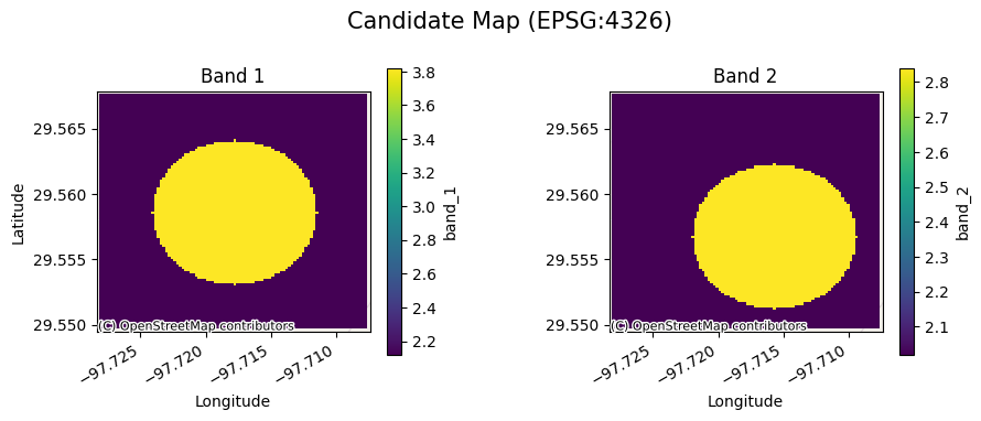
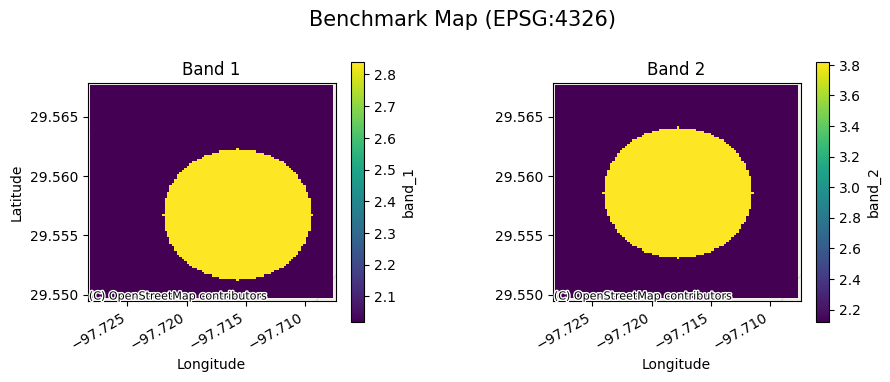
[5]:
cds = rxr.open_rasterio(f'{data_path}/candidate_continuous_1.tif', band_as_variable=True, mask_and_scale=True)
bds = rxr.open_rasterio(f'{data_path}/benchmark_continuous_1.tif', band_as_variable=True, mask_and_scale=True)
[6]:
cds.gval.cont_plot(title="Candidate Map")
[6]:
<matplotlib.collections.QuadMesh at 0x7fa3aac9af50>
[7]:
bds.gval.cont_plot(title="Benchmark Map")
[7]:
<matplotlib.collections.QuadMesh at 0x7fa3aaa6d180>
Let’s use this newly created subsampling dataframe on a continuous comparison. For each subsample an agreement map is created and then used to calculate continuous statistics. There are four subsampling-average types:
full-detail: reports all metrics calculated on separate bands and subsamples.
band: reports all metrics on subsamples with band values averaged.
subsample: reports all metrics on bands with subsample values averaged.
weighted: reports all metrics on bands with subsample values averaged and scaled by weights.
Full-Detail
[8]:
ag, met = cds.gval.continuous_compare(benchmark_map=bds,
                                      metrics=["mean_percentage_error"],
                                      subsampling_df=polygons_continuous,
                                      subsampling_average="full-detail")
met
[8]:
| subsample | band | mean_percentage_error | |
|---|---|---|---|
| 0 | 1 | 1 | 0.125928 |
| 1 | 1 | 2 | -0.111844 |
| 2 | 2 | 1 | 0.167116 |
| 3 | 2 | 2 | -0.143187 |
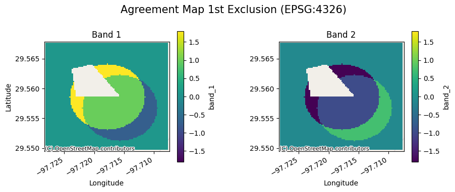
The agreement maps for each subsample will look as follows:
[9]:
ag[0].gval.cont_plot(title="Agreement Map 1st Exclusion")
[9]:
<matplotlib.collections.QuadMesh at 0x7fa3aa732590>
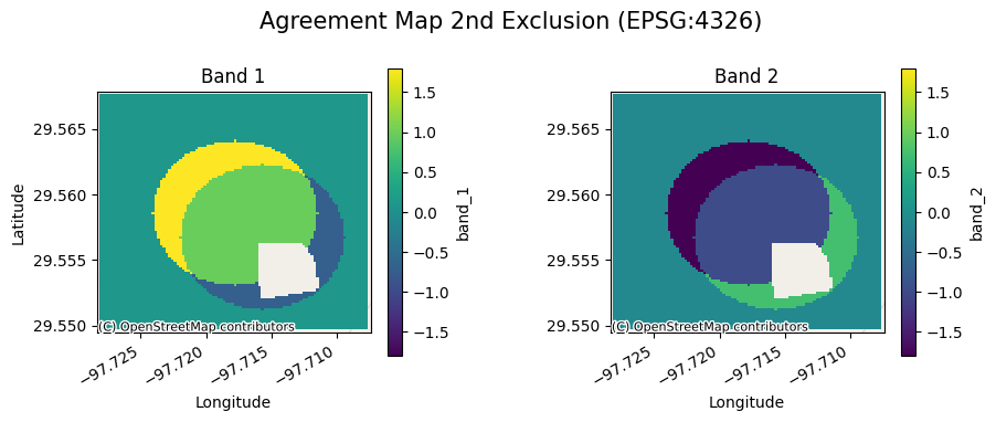
[10]:
ag[1].gval.cont_plot(title="Agreement Map 2nd Exclusion")
[10]:
<matplotlib.collections.QuadMesh at 0x7fa3aa6e5cc0>
Band
[11]:
ag, met = cds.gval.continuous_compare(benchmark_map=bds,
                                      metrics=["mean_percentage_error"],
                                     subsampling_df=polygons_continuous,
                                     subsampling_average="band")
met
[11]:
| subsample | band | mean_percentage_error | |
|---|---|---|---|
| 0 | 1 | averaged | 0.007042 |
| 1 | 2 | averaged | 0.011964 |
Subsample
[12]:
ag, met = cds.gval.continuous_compare(benchmark_map=bds,
                                      metrics=["mean_percentage_error"],
                                     subsampling_df=polygons_continuous,
                                     subsampling_average="subsample")
met
[12]:
| subsample | band | mean_percentage_error | |
|---|---|---|---|
| 0 | averaged | 1 | 0.146522 |
| 1 | averaged | 2 | -0.127515 |
Weighted
[13]:
ag, met = cds.gval.continuous_compare(benchmark_map=bds,
                                      metrics=["mean_percentage_error"],
                                      subsampling_df=polygons_continuous,
                                      subsampling_average="weighted")
met
[13]:
| subsample | band | mean_percentage_error | |
|---|---|---|---|
| 0 | averaged | 1 | 0.083952 |
| 1 | averaged | 2 | -0.037281 |
If one desires to have only one subsample with all of the exclusions combined use Shapely’s unary_union:
[14]:
combined_df = gpd.GeoDataFrame(geometry=[unary_union(polygons_continuous['geometry'])],
                               crs=polygons_continuous.crs)
combined_df.gval.create_subsampling_df(subsampling_type=["exclude"], inplace=True)
ag, met = cds.gval.continuous_compare(benchmark_map=bds,
                                      metrics=["mean_percentage_error"],
                                      subsampling_df=combined_df,
                                      subsampling_average="full-detail")
met
[14]:
| subsample | band | mean_percentage_error | |
|---|---|---|---|
| 0 | 1 | 1 | 0.133122 |
| 1 | 1 | 2 | -0.117482 |
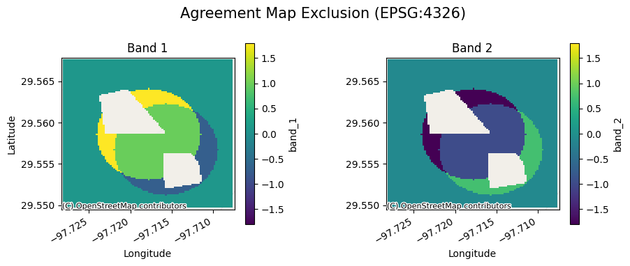
[15]:
ag[0].gval.cont_plot(title="Agreement Map Exclusion")
[15]:
<matplotlib.collections.QuadMesh at 0x7fa3aa4e0820>
Categorical
[16]:
# Subsampling DF
polygons_categorical = gpd.read_file(f'{data_path}/subsample_two-class_polygons.gpkg')
polygons_categorical.gval.create_subsampling_df(subsampling_type=["include", "include"], inplace=True)
polygons_categorical.explore()
[16]:
[17]:
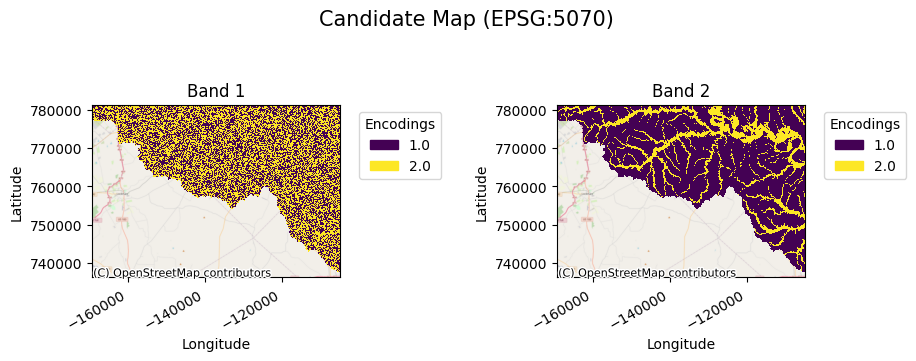
# Candidate and Benchmark
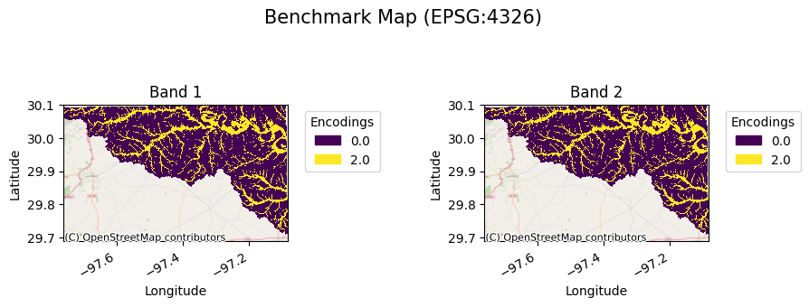
cda = rxr.open_rasterio(f'{data_path}/candidate_map_multiband_two_class_categorical.tif', mask_and_scale=True)
bda = rxr.open_rasterio(f'{data_path}/benchmark_map_multiband_two_class_categorical.tif', mask_and_scale=True)
[18]:
cda.gval.cat_plot("Candidate Map")
[18]:
<matplotlib.collections.QuadMesh at 0x7fa399f6e290>
[19]:
bda.gval.cat_plot("Benchmark Map")
[19]:
<matplotlib.collections.QuadMesh at 0x7fa38a781ba0>
Just as done earlier in continuous comparison, the following performs subsampling on categorical comparisons.. For each subsample an agreement map, a cross-tabulation table, and a metric table is created. There are three subsampling-average types:
full-detail: reports all metrics calculated on separate bands and subsamples.
band: reports all metrics on subsamples with band values averaged.
subsample: reports all metrics on bands with subsample values averaged.
Full-detail
[20]:
ag, ctab, met = cda.gval.categorical_compare(benchmark_map=bda,
                                             metrics="all",
                                             positive_categories=[2],
                                             negative_categories=[0, 1],
                                             subsampling_df=polygons_categorical,
                                             subsampling_average="full-detail")
met.transpose()
[20]:
| 0 | 1 | 2 | 3 | |
|---|---|---|---|---|
| band | 1 | 1 | 2 | 2 |
| subsample | 1 | 2 | 1 | 2 |
| fn | 201953.0 | 182389.0 | 68239.0 | 58638.0 |
| fp | 761242.0 | 397531.0 | 43646.0 | 65967.0 |
| tn | 762262.0 | 398338.0 | 1479858.0 | 729902.0 |
| tp | 201936.0 | 181301.0 | 335650.0 | 305052.0 |
| accuracy | 0.50026 | 0.499879 | 0.94195 | 0.892541 |
| balanced_accuracy | 0.500157 | 0.499506 | 0.901198 | 0.877941 |
| critical_success_index | 0.173316 | 0.238171 | 0.749997 | 0.70999 |
| equitable_threat_score | 0.000104 | -0.000426 | 0.696008 | 0.602268 |
| f_score | 0.29543 | 0.384715 | 0.857141 | 0.830402 |
| false_discovery_rate | 0.790344 | 0.686781 | 0.115071 | 0.1778 |
| false_negative_rate | 0.500021 | 0.501496 | 0.168955 | 0.161231 |
| false_omission_rate | 0.209448 | 0.31407 | 0.044079 | 0.074363 |
| false_positive_rate | 0.499665 | 0.499493 | 0.028648 | 0.082887 |
| fowlkes_mallows_index | 0.323765 | 0.395147 | 0.857564 | 0.830444 |
| matthews_correlation_coefficient | 0.000255 | -0.000918 | 0.821398 | 0.751849 |
| negative_likelihood_ratio | 0.999373 | 1.001976 | 0.173938 | 0.175802 |
| negative_predictive_value | 0.790552 | 0.68593 | 0.955921 | 0.925637 |
| overall_bias | 2.384759 | 1.591553 | 0.93911 | 1.020152 |
| positive_likelihood_ratio | 1.000628 | 0.99802 | 29.0084 | 10.119461 |
| positive_predictive_value | 0.209656 | 0.313219 | 0.884929 | 0.8222 |
| prevalence | 0.209552 | 0.313645 | 0.209552 | 0.313645 |
| prevalence_threshold | 0.499922 | 0.500248 | 0.156594 | 0.239171 |
| true_negative_rate | 0.500335 | 0.500507 | 0.971352 | 0.917113 |
| true_positive_rate | 0.499979 | 0.498504 | 0.831045 | 0.838769 |
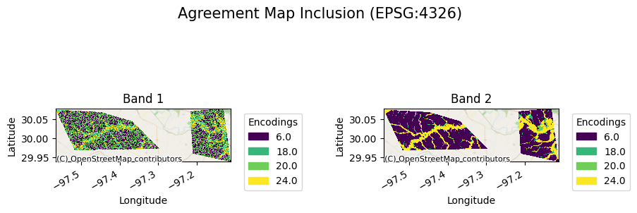
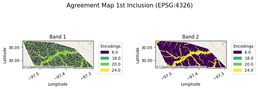
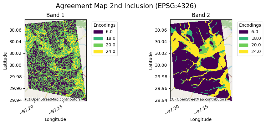
The agreement map will look as follows:
[21]:
ag[0].gval.cat_plot(title="Agreement Map 1st Inclusion")
[21]:
<matplotlib.collections.QuadMesh at 0x7fa39a335600>
[23]:
ag[1].gval.cat_plot(title="Agreement Map 2nd Inclusion")
[23]:
<matplotlib.collections.QuadMesh at 0x7fa3a6fa5d80>
Band
[24]:
ag, ctab, met = cda.gval.categorical_compare(benchmark_map=bda,
                                             metrics="all",
                                             positive_categories=[2],
                                             negative_categories=[0, 1],
                                             subsampling_df=polygons_categorical,
                                             subsampling_average="band")
met.transpose()
[24]:
| 0 | 1 | |
|---|---|---|
| subsample | 1 | 2 |
| band | averaged | averaged |
| fn | 270192.0 | 241027.0 |
| fp | 804888.0 | 463498.0 |
| tn | 2242120.0 | 1128240.0 |
| tp | 537586.0 | 486353.0 |
| accuracy | 0.721105 | 0.69621 |
| balanced_accuracy | 0.700678 | 0.688723 |
| critical_success_index | 0.333352 | 0.408399 |
| equitable_threat_score | 0.192488 | 0.211025 |
| f_score | 0.500021 | 0.579948 |
| false_discovery_rate | 0.599556 | 0.487969 |
| false_negative_rate | 0.334488 | 0.331363 |
| false_omission_rate | 0.107547 | 0.176026 |
| false_positive_rate | 0.264157 | 0.29119 |
| fowlkes_mallows_index | 0.516237 | 0.585118 |
| matthews_correlation_coefficient | 0.342864 | 0.356123 |
| negative_likelihood_ratio | 0.454564 | 0.467492 |
| negative_predictive_value | 0.892453 | 0.823974 |
| overall_bias | 1.661934 | 1.305853 |
| positive_likelihood_ratio | 2.519382 | 2.296222 |
| positive_predictive_value | 0.400444 | 0.512031 |
| prevalence | 0.209552 | 0.313645 |
| prevalence_threshold | 0.38651 | 0.397562 |
| true_negative_rate | 0.735843 | 0.70881 |
| true_positive_rate | 0.665512 | 0.668637 |
Subsample
[25]:
ag, ctab, met = cda.gval.categorical_compare(benchmark_map=bda,
                                             metrics="all",
                                             positive_categories=[2],
                                             negative_categories=[0, 1],
                                             subsampling_df=polygons_categorical,
                                             subsampling_average="subsample")
met.transpose()
[25]:
| 0 | 1 | |
|---|---|---|
| subsample | averaged | averaged |
| band | 1 | 2 |
| fn | 384342.0 | 126877.0 |
| fp | 1158773.0 | 109613.0 |
| tn | 1160600.0 | 2209760.0 |
| tp | 383237.0 | 640702.0 |
| accuracy | 0.500117 | 0.92339 |
| balanced_accuracy | 0.499837 | 0.893723 |
| critical_success_index | 0.198944 | 0.730401 |
| equitable_threat_score | -0.000122 | 0.657571 |
| f_score | 0.331866 | 0.844199 |
| false_discovery_rate | 0.751469 | 0.146089 |
| false_negative_rate | 0.50072 | 0.165295 |
| false_omission_rate | 0.248774 | 0.054299 |
| false_positive_rate | 0.499606 | 0.04726 |
| fowlkes_mallows_index | 0.352259 | 0.844253 |
| matthews_correlation_coefficient | -0.000282 | 0.793505 |
| negative_likelihood_ratio | 1.000651 | 0.173494 |
| negative_predictive_value | 0.751226 | 0.945701 |
| overall_bias | 2.008927 | 0.977509 |
| positive_likelihood_ratio | 0.999348 | 17.662067 |
| positive_predictive_value | 0.248531 | 0.853911 |
| prevalence | 0.248653 | 0.248653 |
| prevalence_threshold | 0.500082 | 0.192211 |
| true_negative_rate | 0.500394 | 0.95274 |
| true_positive_rate | 0.49928 | 0.834705 |
As done earlier, if one wants to combine the inclusion of multiple polygons use unary_union:
[26]:
combined_df = gpd.GeoDataFrame(geometry=[unary_union(polygons_categorical['geometry'])],
                               crs=polygons_continuous.crs)
combined_df.gval.create_subsampling_df(subsampling_type=["include"], inplace=True)
ag, ctab, met = cda.gval.categorical_compare(benchmark_map=bda,
                                             metrics="all",
                                             positive_categories=[2],
                                             negative_categories=[0, 1],
                                             subsampling_df=combined_df,
                                             subsampling_average="full-detail")
met.transpose()
[26]:
| 0 | 1 | |
|---|---|---|
| band | 1 | 2 |
| subsample | 1 | 1 |
| fn | 384342.0 | 126877.0 |
| fp | 1158773.0 | 109613.0 |
| tn | 1160600.0 | 2209760.0 |
| tp | 383237.0 | 640702.0 |
| accuracy | 0.500117 | 0.92339 |
| balanced_accuracy | 0.499837 | 0.893723 |
| critical_success_index | 0.198944 | 0.730401 |
| equitable_threat_score | -0.000122 | 0.657571 |
| f_score | 0.331866 | 0.844199 |
| false_discovery_rate | 0.751469 | 0.146089 |
| false_negative_rate | 0.50072 | 0.165295 |
| false_omission_rate | 0.248774 | 0.054299 |
| false_positive_rate | 0.499606 | 0.04726 |
| fowlkes_mallows_index | 0.352259 | 0.844253 |
| matthews_correlation_coefficient | -0.000282 | 0.793505 |
| negative_likelihood_ratio | 1.000651 | 0.173494 |
| negative_predictive_value | 0.751226 | 0.945701 |
| overall_bias | 2.008927 | 0.977509 |
| positive_likelihood_ratio | 0.999348 | 17.662067 |
| positive_predictive_value | 0.248531 | 0.853911 |
| prevalence | 0.248653 | 0.248653 |
| prevalence_threshold | 0.500082 | 0.192211 |
| true_negative_rate | 0.500394 | 0.95274 |
| true_positive_rate | 0.49928 | 0.834705 |
[27]:
ag[0].gval.cat_plot(title="Agreement Map Inclusion")
[27]:
<matplotlib.collections.QuadMesh at 0x7fa3a1331e40>