Continuous Comparisons

import numpy as np
import xarray as xr
import rioxarray as rxr
import gval

Load Datasets

In this example, the comparisons output of Variable Infiltration Capacity Model total annual CONUS precipitation in 2011 with that of the model output of PRISM, also total annual CONUS precipitation in 2011.

• Livneh B., E.A. Rosenberg, C. Lin, B. Nijssen, V. Mishra, K.M. Andreadis, E.P. Maurer, and D.P. Lettenmaier, 2013: A Long-Term Hydrologically Based Dataset of Land Surface Fluxes and States for the Conterminous United States: Update and Extensions, Journal of Climate, 26, 9384⦣8364;⬓9392. https://psl.noaa.gov/data/gridded/data.livneh.html

• PRISM Climate Group, Oregon State University, https://prism.oregonstate.edu, data created 4 Feb 2014, accessed 16 Dec 2020. https://prism.oregonstate.edu/recent/

candidate = rxr.open_rasterio(
    './livneh_2011_precip.tif', mask_and_scale=True
) # VIC
benchmark = rxr.open_rasterio(
    './prism_2011_precip.tif', mask_and_scale=True
) # PRISM

Run GVAL Continuous Compare

agreement, metric_table = candidate.gval.continuous_compare(benchmark)

Output

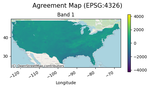
Agreement Map

The agreement map in this case will be simply the difference between the two modeling outputs.

agreement.gval.cont_plot(title="Agreement Map", figsize=(6, 3))

<matplotlib.collections.QuadMesh at 0x7f01f38bba60>

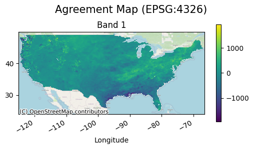
In this case it is a bit difficult to see the variability of the precipitation difference, but if extreme values are masked out the map will look like the following:

agreement.data = xr.where(
    (agreement < np.nanquantile(agreement.values, 0.0001)) |
    (agreement > np.nanquantile(agreement.values, 0.9999)),
    np.nan,
    agreement
)
agreement.gval.cont_plot(title="Agreement Map", figsize=(6, 3))

<matplotlib.collections.QuadMesh at 0x7f01f385b430>

Metric Table

A metric table contains information about the unit of analysis, (a single band in this case), and selected continuous metrics. Since we did not provide the metrics argument GVAL computed all of the available continuous statistics.

metric_table.transpose()

	0
band	1
coefficient_of_determination	0.685261
mean_absolute_error	216.089706
mean_absolute_percentage_error	0.319234
mean_normalized_mean_absolute_error	0.267845
mean_normalized_root_mean_squared_error	0.372578
mean_percentage_error	0.010022
mean_signed_error	8.085411
mean_squared_error	90351.664062
range_normalized_mean_absolute_error	0.033065
range_normalized_root_mean_squared_error	0.045995
root_mean_squared_error	300.585541
symmetric_mean_absolute_percentage_error	0.269394

Alternative Uses of GVAL Continuous Operations

Aside form running the entire process, it is possible to run each of the following steps individually: homogenizing maps, computing an agreement map. This allows for flexibility in workflows so that a user may use as much or as little functionality as needed.

Just like in continuous comparisons, homogenizing can be done as follows:

candidate, benchmark = candidate.gval.homogenize(
    benchmark_map=benchmark,
    target_map = "candidate"
)

The “difference” comparison function is the default used for the comparison_function argument in gval.continuous_compare and is the only continuous comparison function available by default. It would be advised not to use a categorical comparison function such as ‘cantor’, ‘szudzik’, or a pairing dicitonary because it could result in a very large number of classes.

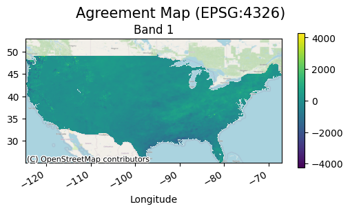
Using difference in comparison:

agreement_map = candidate.gval.compute_agreement_map(
    benchmark_map=benchmark,
    comparison_function="difference",
    continuous=True
)

agreement_map.gval.cont_plot(title="Agreement Map", figsize=(6, 3))

<matplotlib.collections.QuadMesh at 0x7f01f37525c0>

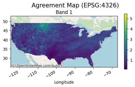
The following uses an abritrary custom registered function for use in a continuous agreement map:

from gval import Comparison
from numbers import Number

@Comparison.register_function(name='divide', vectorize_func=True)
def multiply(c: Number, b: Number) -> Number:
    return c / b

agreement_map = candidate.gval.compute_agreement_map(
    benchmark_map=benchmark,
    comparison_function="divide",
    continuous=True
)

agreement_map.gval.cont_plot(title="Agreement Map", figsize=(6, 3))

<matplotlib.collections.QuadMesh at 0x7f01f3635cc0>

Like in cateogrical compare, all metrics are computed by default if no argument is provided, metrics can also take a list of the desired metrics and will only return metrics in this list.

_, metric_table = candidate.gval.continuous_compare(
    benchmark,
    metrics=['mean_absolute_error', 'mean_squared_error']
)

metric_table

	band	mean_absolute_error	mean_squared_error
0	1	215.106232	89814.117188

Just like registering comparison functions, you are able to register a metric function on both a method and a class of functions. Below is registering a metric function:

from typing import Union
import numpy as np
import xarray as xr
from gval import ContStats

@ContStats.register_function(name="min_error")
def min_error(error: Union[xr.Dataset, xr.DataArray]) -> float:
    return error.min().values

The following is registering a class of metric functions. In this case, the names associated with each function will respond to each method’s name.

@ContStats.register_function_class()
class MetricFunctions:

    @staticmethod
    def median_error(error: Union[xr.Dataset, xr.DataArray]) -> float:
        return error.median().values

    @staticmethod
    def max_error(error: Union[xr.Dataset, xr.DataArray]) -> float:
        return error.max().values

_, metric_table = candidate.gval.continuous_compare(
    benchmark,
    metrics=['min_error', 'median_error', 'max_error']
)

metric_table

	band	min_error	median_error	max_error
0	1	-3035.655273	25.858208	4263.23291

Save Output

Finally, a user can take the results and save them to a directory of their choice. The following is an example of saving the agreement map and then the metric table:

# output agreement map
agreement_file = 'continuous_agreement_map.tif'
metric_file = 'continuous_metric_file.csv'

agreement_map.rio.to_raster(agreement_file)
metric_table.to_csv(metric_file)