
Multi-Class Categorical Comparisons
[1]:
import rioxarray as rxr
import gval
import numpy as np
import pandas as pd
import xarray as xr
from itertools import product

pd.set_option('display.max_columns', None)
Load Datasets
[2]:
candidate = rxr.open_rasterio(
    "./candidate_map_multi_categorical.tif", mask_and_scale=True
)
benchmark = rxr.open_rasterio(
    "./benchmark_map_multi_categorical.tif", mask_and_scale=True
)
depth_raster = rxr.open_rasterio(
    "./candidate_raw_elevation_multi_categorical.tif", mask_and_scale=True
)
Homogenize Datasets and Make Agreement Map
Although one can call candidate.gval.categorical_compare to run the entire workflow, in this case homogenization and creation of an agreement map will be done separately to show more options for multi-class comparisons.
Homogenize
[3]:
candidate_r, benchmark_r = candidate.gval.homogenize(benchmark)
depth_raster_r, arb = depth_raster.gval.homogenize(benchmark_r)
del arb
Agreement Map
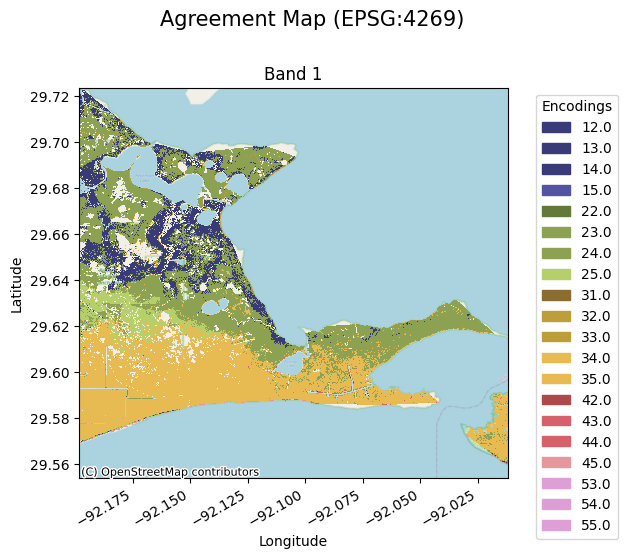
The following makes a pairing dictionary which maps combinations of values in the candidate and benchmark maps to unique values in the agreement map. In this case we will encode each value as concatenation of what the values are. Instead of making a pairing dictionary one can use the szudzik or cantor pairing functions to make unique values for each combination of candidate and benchmark map values. e.g. 12 represents a class 1 for the candidate and a class 2 for the benchmark.
[4]:
classes = [1, 2, 3, 4, 5]
pairing_dictionary = {(x, y): int(f'{x}{y}') for x, y in product(*([classes]*2))}

# Showing the first 6 entries
print('\n'.join([f'{k}: {v}' for k,v  in pairing_dictionary.items()][:6]))
(1, 1): 11
(1, 2): 12
(1, 3): 13
(1, 4): 14
(1, 5): 15
(2, 1): 21
The benchmark map has an extra class 0 which is very similar to nodata so it will not be included in allow_benchmark_values in the following methods.
[5]:
agreement_map = candidate_r.gval.compute_agreement_map(
    benchmark_r,
    nodata=255,
    encode_nodata=True,
    comparison_function="pairing_dict",
    pairing_dict=pairing_dictionary,
    allow_candidate_values=classes,
    allow_benchmark_values=classes,
)

crosstab = agreement_map.gval.compute_crosstab()
The following only shows a small subset of the map for memory purposes:
[7]:
agreement_map.gval.cat_plot(
    title='Agreement Map',
    figsize=(8, 6),
    colormap='tab20b'
)
[7]:
<matplotlib.collections.QuadMesh at 0x7f99a1e34b50>
Comparisons
For multi-categorical statistics GVAL offers 4 methods of averaging:
No Averaging which provides one vs. all metrics on a class basis
Micro Averaging which sums up the contingencies of each class defined as either positive or negative
Macro Averaging which sums up the contingencies of one class vs all and then averages them
Weighted Averaging which does macro averaging with the inclusion of weights to be applied to each positive category.
Using None for the averaging argument runs a one class vs. all methodology for each class and reports their metrics on a class basis:
[8]:
no_averaged_metrics = crosstab.gval.compute_categorical_metrics(
    positive_categories=[1, 2, 3, 4, 5],
    negative_categories=None,
    average=None
)
no_averaged_metrics.transpose()
[8]:
| 0 | 1 | 2 | 3 | 4 | |
|---|---|---|---|---|---|
| band | 1 | 1 | 1 | 1 | 1 |
| positive_categories | 1 | 2 | 3 | 4 | 5 |
| fn | 6.0 | 1043.0 | 318274.0 | 516572.0 | 364147.0 |
| fp | 172762.0 | 561004.0 | 462496.0 | 3775.0 | 5.0 |
| tn | 1043592.0 | 653360.0 | 422623.0 | 693617.0 | 852206.0 |
| tp | 0.0 | 953.0 | 12967.0 | 2396.0 | 2.0 |
| accuracy | 0.857963 | 0.537927 | 0.358109 | 0.57221 | 0.700622 |
| balanced_accuracy | 0.428984 | 0.507741 | 0.258311 | 0.499602 | 0.5 |
| critical_success_index | 0.0 | 0.001693 | 0.016337 | 0.004584 | 0.000005 |
| equitable_threat_score | -0.000005 | 0.000055 | -0.175401 | -0.000455 | -0.0 |
| f_score | 0.0 | 0.00338 | 0.032148 | 0.009125 | 0.000011 |
| false_discovery_rate | 1.0 | 0.998304 | 0.972728 | 0.611732 | 0.714286 |
| false_negative_rate | 1.0 | 0.522545 | 0.960853 | 0.995383 | 0.999995 |
| false_omission_rate | 0.000006 | 0.001594 | 0.429579 | 0.426852 | 0.299376 |
| false_positive_rate | 0.142033 | 0.461974 | 0.522524 | 0.005413 | 0.000006 |
| fowlkes_mallows_index | 0.0 | 0.028455 | 0.032675 | 0.042339 | 0.001253 |
| matthews_correlation_coefficient | -0.000904 | 0.001257 | -0.440983 | -0.005543 | -0.000072 |
| negative_likelihood_ratio | 1.165546 | 0.971226 | 2.01236 | 1.000801 | 1.0 |
| negative_predictive_value | 0.999994 | 0.998406 | 0.570421 | 0.573148 | 0.700624 |
| overall_bias | 28793.666667 | 281.541583 | 1.435399 | 0.011891 | 0.000019 |
| positive_likelihood_ratio | 0.0 | 1.033511 | 0.074919 | 0.852916 | 0.936112 |
| positive_predictive_value | 0.0 | 0.001696 | 0.027272 | 0.388268 | 0.285714 |
| prevalence | 0.000005 | 0.001641 | 0.272322 | 0.426657 | 0.299376 |
| prevalence_threshold | 1.0 | 0.49588 | 0.785107 | 0.519876 | 0.508252 |
| true_negative_rate | 0.857967 | 0.538026 | 0.477476 | 0.994587 | 0.999994 |
| true_positive_rate | 0.0 | 0.477455 | 0.039147 | 0.004617 | 0.000005 |
The following is an example of a using micro averaging to combine classes to process two-class categorical statistics. In this example we will use classes 1 and 2 as positive classes and classes 3, 4, and 5 as negative classes:
[9]:
micro_averaged_metrics = crosstab.gval.compute_categorical_metrics(
    positive_categories=[1, 2],
    negative_categories=[3, 4, 5],
    average="micro"
)
micro_averaged_metrics.transpose()
[9]:
| 0 | |
|---|---|
| band | 1 |
| fn | 382.0 |
| fp | 733099.0 |
| tn | 481259.0 |
| tp | 1620.0 |
| accuracy | 0.396987 |
| balanced_accuracy | 0.602749 |
| critical_success_index | 0.002204 |
| equitable_threat_score | 0.00056 |
| f_score | 0.004398 |
| false_discovery_rate | 0.997795 |
| false_negative_rate | 0.190809 |
| false_omission_rate | 0.000793 |
| false_positive_rate | 0.603693 |
| fowlkes_mallows_index | 0.04224 |
| matthews_correlation_coefficient | 0.017033 |
| negative_likelihood_ratio | 0.481468 |
| negative_predictive_value | 0.999207 |
| overall_bias | 366.992507 |
| positive_likelihood_ratio | 1.340402 |
| positive_predictive_value | 0.002205 |
| prevalence | 0.001646 |
| prevalence_threshold | 0.463444 |
| true_negative_rate | 0.396307 |
| true_positive_rate | 0.809191 |
The following shows macro averaging and is equivalent to the values of shared columns in no_averaged_comps.mean():
[10]:
macro_averaged_metrics = crosstab.gval.compute_categorical_metrics(
    positive_categories=classes,
    negative_categories=None,
    average="macro"
)
macro_averaged_metrics.transpose()
[10]:
| 0 | |
|---|---|
| band | 1 |
| accuracy | 0.605366 |
| balanced_accuracy | 0.438927 |
| critical_success_index | 0.004524 |
| equitable_threat_score | -0.035161 |
| f_score | 0.008933 |
| false_discovery_rate | 0.85941 |
| false_negative_rate | 0.895755 |
| false_omission_rate | 0.231481 |
| false_positive_rate | 0.22639 |
| fowlkes_mallows_index | 0.020944 |
| matthews_correlation_coefficient | -0.089249 |
| negative_likelihood_ratio | 1.229986 |
| negative_predictive_value | 0.768519 |
| overall_bias | 5815.331112 |
| positive_likelihood_ratio | 0.579492 |
| positive_predictive_value | 0.14059 |
| prevalence | 0.2 |
| prevalence_threshold | 0.661823 |
| true_negative_rate | 0.77361 |
| true_positive_rate | 0.104245 |
To further enhance macro-averaging, we can apply weights to the classes of interest in order to appropriately change the strength of evaluations for each class. For instance, if we applied the following vector the classes uses in this notebook, [1, 4, 1, 5, 1], classes 2 and 4 would have greater influence on the final averaging of the scores for all classes. (All weight values are in reference to the other weight values respectively. e.g. the vector [5, 5, 5, 5, 5] would cause no
change in the averaging because each weight value is equivalent to a ll other weight values.) Let’s use the first weight vector mentioned in weighted averaging:
[11]:
weight_averaged_metrics = crosstab.gval.compute_categorical_metrics(
    positive_categories=classes,
    weights=[1, 4, 1, 5, 1],
    negative_categories=None,
    average="weighted"
)
weight_averaged_metrics.transpose()
[11]:
| 0 | |
|---|---|
| band | 1 |
| accuracy | 0.577454 |
| balanced_accuracy | 0.476356 |
| critical_success_index | 0.003836 |
| equitable_threat_score | -0.014789 |
| f_score | 0.007609 |
| false_discovery_rate | 0.811574 |
| false_negative_rate | 0.835662 |
| false_omission_rate | 0.239133 |
| false_positive_rate | 0.211627 |
| fowlkes_mallows_index | 0.029953 |
| matthews_correlation_coefficient | -0.03872 |
| negative_likelihood_ratio | 1.088901 |
| negative_predictive_value | 0.760867 |
| overall_bias | 2493.443989 |
| positive_likelihood_ratio | 0.784138 |
| positive_predictive_value | 0.188426 |
| prevalence | 0.225962 |
| prevalence_threshold | 0.573022 |
| true_negative_rate | 0.788373 |
| true_positive_rate | 0.164338 |
Regardless of the averaging methodology it seems as though the candidate does not agree with the benchmark. We can now save the output.
Save Output
[12]:
# output agreement map
agreement_file = 'multi_categorical_agreement_map.tif'
metric_file = 'macro_averaged_metric_file.csv'

agreement_map.rio.to_raster(agreement_file)
macro_averaged_metrics.to_csv(metric_file)