Background

The hydrofabric team is focused on delivering a consistent, interoperable, flexible, cloud native solution for hydrofabric data to those interested in hydrologic modeling and geospatial analysis. We aim to provide open data to improve open science and it doing so strive to make real data FAIR data.

In the contexts of DevCon, the hydrofabric provides the foundational features, topology and attributes needed for cartography, web mapping, geospatial analysis, machine learning, model evaluation, data assimilation, and NextGen (and AWI data stream, NGIAB, etc) applications. Outside of DevCon, it provides the needed infrastructure to support other mutli-scale modeling needs (e.g. NHM, US Water Census, Water Balance), vulnerability assessments, and more!

Background

Last year, we shared the concept of a hydrofabric and the current of NextGen data structures. A hydrofabric describes the landscape and flow network discretizations, the essential connectivity of network features, and the key reporting locations known as nexus points. Combined these feature serve as both geospatail and computational elements that allow the NextGen modeling infrastructure to syncronious different models, formulations, and domains into a cohert simulation and set of outputs.

Key Highlights

1. Design Philosophy: We adopt the OGC HY Feature conceptual model with custom modifications for NextGen applications that define an explicit data model. This fundamental data model and evolving mode of delevery tailored for modeling and web infrastructure applications, emphasizing efficiency and accuracy through use of modern geospatial and data science formats. This included seven spatial and two a-spatial layers, and future plans for an additional layer for water bodies and cross sections. The NOAA enterprise hydrofabric is made up of 5 modular components, all of which will be touched on today. These include those seen below:

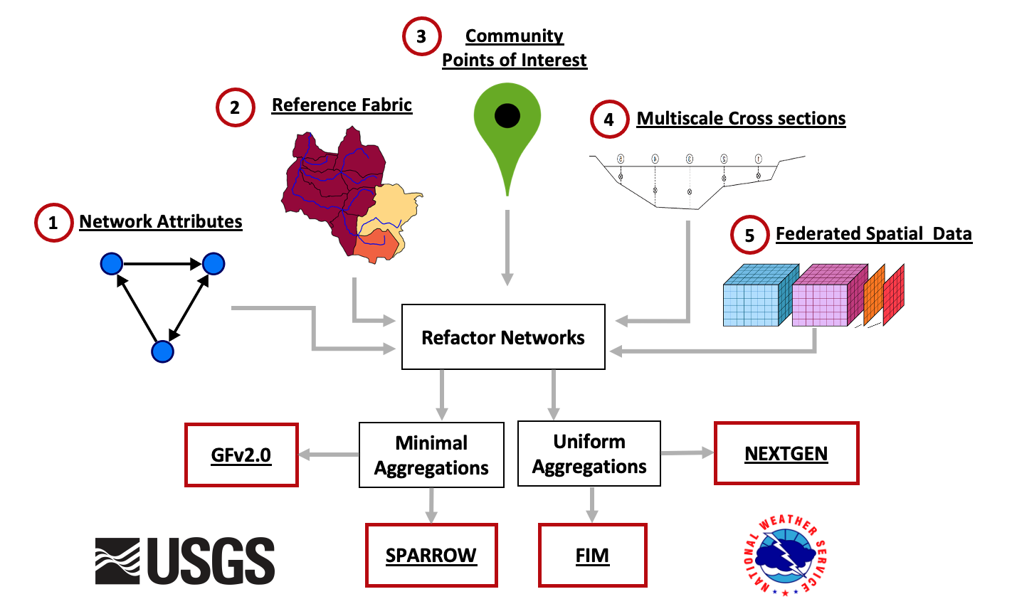
Enterprise Hydrofabric System

2. NHGF: A core, federally consistent data product grounded in a common topology, reference fabric, and set of community POIs. Collectively, these define a shared NOAA/USGS National Hydrologic Geospatial Fabric (NHGF).

3. Network Manipulation: In-depth exploration of two network manipulation processes, refactoring and aggregating, that are crucial for optimizing data usage.

4. Egress Free Community Hydrofabric Data: Through Lynker-Spatial we provide efficient, free access to hydrofabric and hydrofabric-adjacent data. Over the last year, this system has had ~78,500 requests over 2,306 unique IPs with a month over month trend nearing exponential.

5. Data Subsetting: We demonstrated methods to extract data subsets for multi-scale modeling tasks using R and a Go-based CLI. Since then, the R version and underlying data stores have been overhauled, the CLI implementation has transitioned to a (beta) REST API, and a Python implementation is forthcoming.

6. Enriching a hydrofabric: While the core hydrofabric respects the above data model we demontrated hoe it could be enhance through te addtioon of catchment attributes (both precomputed and custom), flowpath attributes, and forcing weights. Since then, through a partnership with ESIP we extended the climateR catalog to host access endpoints to over 100,000 unique data resources, developed a e machine learning models for estimating river bathymety and roughness, tools to extract high resolution bathymetry informed ross sections, and applid these across CONUS - all of which are provided in the egress free cloud resources!

Software

While the primary output of this system is a constantly evolving FAIR, cloud native, data products complete with services, these are all predicated on a suite of research (hydrofab) to publication ready (nhdplusTools, climateR) software. This suite of software is bundled together in NOAA-OWP/hydrofabric provides a collection of R packages designed for hydroscience data development and access. These packages share an underlying design philosophy, grammar, and data structures, making them easier to apply together. The packages cover a wide range of data manipulation tasks, from importing and cleaning data, to building custom hydrofabrics, to accessing and summarizing data from 100,000’s of data resources. Assuming you are already up and running with R, RStudio, and hydrofabric, you can attach the library to a working session:

library(hydrofabric)

library(hydrofabric) will load the core packages (alphabetical):

• climateR for accessing federated data stores for parameter and attributes estimation
• hfsubsetR for cloud-based hydrofabric subsetting
• hydrofab a tool set for “fabricating” multiscale hydrofabrics
• ngen.hydrofab NextGen extensions for hydrofab
• nhdplusTools for network manipulation
• zonal for catchment parameter estimation

Additionally it will load key geospatial data science libraries:

• dplyr (data.frames)
• sf (vector)
• terra (raster)

Benefits of Using hydrofabric

• Consistency: Packages are designed to work seamlessly together - with the Lynker-Spatial data stores - making workflows more efficient.
• Readability: Syntax is designed to be human-readable and expressive, which helps in writing clean and understandable code.
• Efficiency: Functions are optimized for performance, making data manipulation tasks faster.

Lynker-Spatial Data

Hydrofabric artifacts are generated from a set of federally consistent reference datasets built in collaboration between NOAA, the USGS, and Lynker for federal water modeling efforts. These artifacts are designed to be easily updated, manipulated, and quality controlled to meet the needs of a wide range of modeling tasks while leveraging the best possible input data.

Cloud-native (modified both in structure and format) artifacts of the refactored and aggregated, NextGen ready resources are publicly available through lynker-spatial under an ODbL license. If you use data, please ensure you (1) Attribute Lynker-Spatial, (2) keep the data open, and that (3) any works produced from this data offer that adapted database under the ODbL.

Hydrofabric data on lynker-spatial follows the general s3 URI pattern for access:

"{source}/{version}/{type}/{domain}_{layer}"

Where:

• source is the local or s3 location
• version is the release number (e.g. v2.2)
• type is the type of fabric (e.g. reference, nextgen, etc)
• domain is the region of interest (e.g. conus, hawaii, alaska)
• layer is the layer of the hydrofabric (e.g. divides, flowlines, network, attributes, etc.)

High level Technical Overview

Below we provide more context on the data formats and technology we rely on toe help make our data FAIR, easy to use, and

Data Storage

We use s3 (via aws) for storage that is easy to sync locally, and access remotely. The design of our data structure makes versioning easier to track, and offer parity between local and remote access:

version <- "v2.2"
type <- "reference"
domain <- "conus"

local_source <- "/Users/mjohnson/hydrofabric"
s3_source <- "s3://lynker-spatial/hydrofabric"

# Sync s3 with your local archive
(glue("aws s3 sync {s3_source}/{version}/{type} {local_source}/{version}/{type}"))

## aws s3 sync s3://lynker-spatial/hydrofabric/v2.2/reference /Users/mjohnson/hydrofabric/v2.2/reference

Data Formats

GPKG

Geopackages/SQLITE is an open, standards-based, platform-independent, and data format for spatial . It is designed to be a universal format for geospatial data storage, enabling the sharing and exchange of spatial data across different systems and software.

gpkg <- "tutorial/poudre.gpkg"

# See Layers
st_layers(gpkg)

## Driver: GPKG 
## Available layers:
##   layer_name geometry_type features fields             crs_name
## 1    divides       Polygon     1122      5 NAD83 / Conus Albers
## 2  flowlines   Line String     1129     19 NAD83 / Conus Albers
## 3    network            NA     1145     23                 <NA>

# Read Complete Layer
(divides = read_sf(gpkg, "divides"))

## Simple feature collection with 1122 features and 5 fields
## Geometry type: POLYGON
## Dimension:     XY
## Bounding box:  xmin: -831675 ymin: 1975605 xmax: -757545 ymax: 2061555
## Projected CRS: NAD83 / Conus Albers
## # A tibble: 1,122 × 6
##    divide_id areasqkm has_flowline      id vpuid                            geom
##        <dbl>    <dbl> <lgl>          <dbl> <chr>                   <POLYGON [m]>
##  1   2896607   10.2   TRUE         2896607 10L   ((-779895 2037405, -779835 203…
##  2   2896609    5.08  TRUE         2896609 10L   ((-777075 2041155, -777255 204…
##  3   2897621    0.806 TRUE         2897621 10L   ((-789255 2035395, -789255 203…
##  4   2897627    2.52  TRUE         2897627 10L   ((-802665 2036685, -802755 203…
##  5   2897631    3.23  TRUE         2897631 10L   ((-796005 2034945, -795855 203…
##  6   2897671    1.42  TRUE         2897671 10L   ((-780525 2033175, -780435 203…
##  7   2897731    1.78  TRUE         2897731 10L   ((-776655 2032545, -776775 203…
##  8   2897785    2.93  TRUE         2897785 10L   ((-774765 2032095, -774855 203…
##  9   2897855    1.44  TRUE         2897855 10L   ((-783765 2029515, -783735 202…
## 10   2897893    2.86  TRUE         2897893 10L   ((-774105 2028195, -773985 202…
## # ℹ 1,112 more rows

Arrow/Parquet

Apache Arrow is an open-source project that provides a columnar memory format for flat and hierarchical data. It proviees fast data transfer and processing across different programming languages and platforms without needing to serialize and deserialize the data, making it particularly useful for big data and high-performance applications.

(geo)parquet is an on disc data format for storing columar data. GeoParquet is an emerging standard for storing geospatial data within the Apache Parquet file format. Parquet is a columnar storage file format that is highly efficient for both storage and retrieval, particularly suited for big data and analytics applications.

We distribute hydrofabric layers as VPU-based hive partitioned (geo)parquet stores. These can be accessed from lynker-spatial, or, synced (see above) to a local directory. Hive partitioning is a partitioning strategy that is used to split a table into multiple files based on partition keys. The files are organized into folders.

The complete v2.2/reference/ directory is ~3.0GB while the v2.1.1/nextgen dirctory is ~ 9.0GB (including xs, flowpath/model attributes, forcing weights and routelink)

Parquet store

(x <- glue("{local_source}/{version}/{type}/{domain}_network"))

## /Users/mjohnson/hydrofabric/v2.2/reference/conus_network

(x2 <- open_dataset(x))

## FileSystemDataset with 22 Parquet files
## divide_id: double
## areasqkm: double
## id: double
## toid: double
## terminalpa: double
## mainstemlp: double
## reachcode: string
## frommeas: double
## tomeas: double
## lengthkm: double
## streamorde: double
## totdasqkm: double
## hydroseq: double
## dnhydroseq: double
## outlet_X: double
## outlet_Y: double
## hf_id: double
## topo: string
## poi_id: int32
## hl_link: string
## hl_reference: string
## hl_uri: string
## vpuid: string

glimpse(x2)

## FileSystemDataset with 22 Parquet files
## 2,691,455 rows x 23 columns
## $ divide_id    <double> 869, 881, 885, 897, 899, 903, 905, 907, 911, 923, 925, 9…
## $ areasqkm     <double> 9.8500444, 2.3957955, 3.7908014, 0.8784026, 3.7737083, 1…
## $ id           <double> 869, 881, 885, 897, 899, 903, 905, 907, 911, 923, 925, 9…
## $ toid         <double> 1277, 1383, 1281, 1415, 1371, 901, 909, 1403, 929, 933, …
## $ terminalpa   <double> 1815586, 1815586, 1815586, 1815586, 1815586, 1815586, 18…
## $ mainstemlp   <double> 1819868, 1820217, 1819864, 1820207, 1820178, 1819352, 18…
## $ reachcode    <string> "01020003000346", "01020003000574", "01020003000149", "0…
## $ frommeas     <double> 0.00000, 0.00000, 0.00000, 0.00000, 2.07552, 0.00000, 0.…
## $ tomeas       <double> 100.00000, 100.00000, 100.00000, 100.00000, 100.00000, 5…
## $ lengthkm     <double> 6.2446074, 1.9348602, 4.5941482, 1.1105714, 2.1912820, 1…
## $ streamorde   <double> 1, 1, 2, 2, 1, 3, 1, 3, 3, 1, 1, 2, 1, 1, 1, 3, 1, 3, 1,…
## $ totdasqkm    <double> 9.8379, 5.5125, 32.8410, 4.7736, 3.7440, 46.1160, 4.8789…
## $ hydroseq     <double> 1819868, 1820218, 1819864, 1820208, 1820179, 1820188, 18…
## $ dnhydroseq   <double> 1819867, 1820217, 1819863, 1820207, 1820178, 1820185, 18…
## $ outlet_X     <double> 2122874, 2106010, 2123427, 2101033, 2107853, 2105622, 21…
## $ outlet_Y     <double> 2890039, 2884833, 2889282, 2881567, 2885469, 2882792, 28…
## $ hf_id        <double> 869, 881, 885, 897, 899, 903, 905, 907, 911, 923, 925, 9…
## $ topo         <string> "fl-fl", "fl-fl", "fl-fl", "fl-fl", "fl-fl", "fl-fl", "f…
## $ poi_id        <int32> NA, NA, NA, NA, NA, NA, NA, NA, NA, NA, NA, 4, NA, NA, N…
## $ hl_link      <string> NA, NA, NA, NA, NA, NA, NA, NA, NA, NA, NA, "01020003010…
## $ hl_reference <string> NA, NA, NA, NA, NA, NA, NA, NA, NA, NA, NA, "HUC12", NA,…
## $ hl_uri       <string> NA, NA, NA, NA, NA, NA, NA, NA, NA, NA, NA, "HUC12-01020…
## $ vpuid        <string> "01", "01", "01", "01", "01", "01", "01", "01", "01", "0…

# > Remote parity >
# open_dataset(glue('{s3_source}/{version}/{type}/{domain}_network/'))

Geoparquet store

(x <- glue("{local_source}/{version}/{type}/{domain}_divides"))

## /Users/mjohnson/hydrofabric/v2.2/reference/conus_divides

open_dataset(x)

## FileSystemDataset with 21 Parquet files
## divide_id: double
## areasqkm: double
## geom: binary
## has_flowline: bool
## id: double
## vpuid: string
## 
## See $metadata for additional Schema metadata

# > Renote parity >
# arrow::open_dataset(glue::glue('{s3_source}/{version}/{type}/conus_divides'))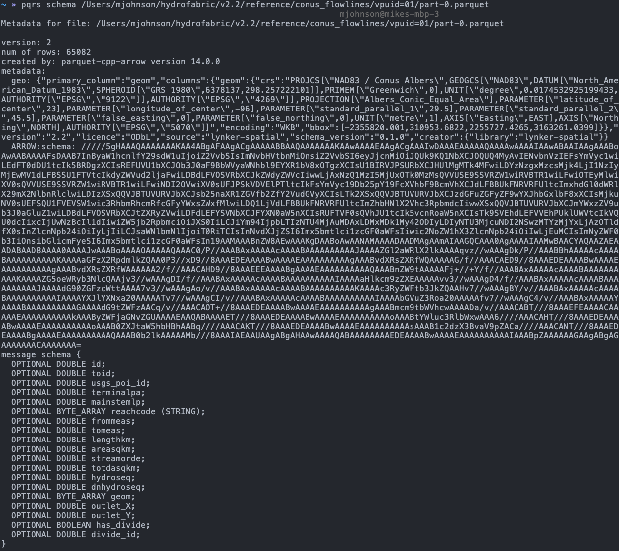

Parquet Schema

The pqrs library offers a command line tool of inspecting Parquet files

pqrs schema /Users/mjohnson/hydrofabric/v2.2/reference/conus_flowlines/vpuid=01/part-0.parquet

Virtual Access to Gridded Data (Primary COG, NetCDF, Zarr)

The amount of gridded data needed for the suite of our supported applications (let alone) - GDAL VSI

"/vsis3/lynker-spatial/gridded-resources/medium_range.forcing.tif" |>
    dap(AOI = divides) |>
    plot()

Lazy Evaluation

All datasets are distributed at the domain level (e.g. conus, hawaii, alaska). Lazy evaluation can help you get just the data you need, in memory from local or remote locations.

Local GPKG

as_sqlite(gpkg, "divides") %>%
    filter(divide_id == 2896607)

## # Source:   SQL [1 x 7]
## # Database: sqlite 3.45.2 [/Users/mjohnson/github/hydrofabric/vignettes/tutorial/poudre.gpkg]
##     fid          geom divide_id areasqkm has_flowline      id vpuid
##   <int>        <blob>     <dbl>    <dbl>        <int>   <dbl> <chr>
## 1     1 <raw 2.21 kB>   2896607     10.2            1 2896607 10L

as_sqlite(gpkg, "divides") %>%
    filter(divide_id == 2896607) %>%
    read_sf_dataset_sqlite()

## Simple feature collection with 1 feature and 6 fields
## Geometry type: POLYGON
## Dimension:     XY
## Bounding box:  xmin: -780615 ymin: 2037165 xmax: -777075 ymax: 2044425
## Projected CRS: NAD83 / Conus Albers
## # A tibble: 1 × 7
##     fid                        geom divide_id areasqkm has_flowline     id vpuid
## * <int>               <POLYGON [m]>     <dbl>    <dbl>        <int>  <dbl> <chr>
## 1     1 ((-779895 2037405, -779835…   2896607     10.2            1 2.90e6 10L

Local/Remote Parquet Store

open_dataset(glue("{local_source}/{version}/{type}/conus_network/")) %>%
    filter(id == 101) %>%
    select(id, toid) %>%
    collect()

## # A tibble: 1 × 2
##      id    toid
##   <dbl>   <dbl>
## 1   101 1078719

# >
# arrow::open_dataset(glue::glue('{s3_source}/{version}/{type}/conus_network/'))
# %>% > dplyr::filter(id == 101) %>% > dplyr::select(id,
# toid) %>% > dplyr::collect()

Extracting a VPU

Last year we highlighted a system that was built largely around VPU level gpkgs. While we no longer distribute these files, there is a utility function hfsubsetR::get_vpu_fabric that will extract a VPU level GPKG to a outfile of choice.

get_vpu_fabric("01", type = "reference", hf_version = "2.2",
    outfile = "/Users/mjohnson/Downloads/01_ref_2.2.gpkg")

## [1] "/Users/mjohnson/Downloads/01_ref_2.2.gpkg"

oCONUS domains

We are slowly building up our oCONIS (Ontario, HI, PRVI, AK) domains. As they become avaialble, the same logic above will apply. For example to get Hawaii divides:

open_dataset(glue("{local_source}/{version}/{type}/hawaii_flowlines")) %>%
    read_sf_dataset() %>%
    mapview::mapview()