Realizations and Views

TL;DR

realization -> identification and concepts
view -> representation and operations

Intro

The NextGen Hydrofabric Data Model aims to support a multi-realization view of the river network and landscape using the concepts outlined in the OGC HY Features Standard.

The data model we are proposing, and enforcing, is aimed to allow flexible realizations with minimal data I/O. It does this by

Defining a principle realization,
Storing multiple layers of data in a self contained data format.
Using opaque identifiers to reference realizations of the same hydrologic unit across layers

NOTE: All layers in the GPKG are realizations of the hydrologic landscape. Ultimetly there is one principle realization that defines the principle unit (e.g. flowpath) of the hydrologic landscape per the model application being targeted. Moreover, one is a viewed realization - that is - the one that is being operated on. These do not have to be the same.concpets of

The definition of a view - which is outside of the HY Features spec - is needed when applying concrete representations of the abstract conceptual features. Fundamentally, the way the world is digitally represented dictates the types of operations, inquires, and analysis that can be done and aligning the aims of these analysis, with a view of the abstract hydrologic feature, is critical for efficiency.

NextGen

The notion of a HY Feature ready hydrofabric requires the ability to access a number of realizations. This is distinct from the reference fabric which is intended to support the creation of data products that serve a range of modeling applications. In its current state, NextGen requires a few realizations for model execution. This currently includes, but is likely not limited to, the following:

	Task	Realization	Attributes	Example
1	Forcing Engine	Divide complex with geometry	`divide_id`, `geometry`	Rescale gridded data to units of divide complex
2	Rainfall Runoff Modeling	Divide complex without geometry	`divide_id`, `id`	Linking divide units to draining flowpath
3	Routing	Flowpath network	`id`, `toid`	Moving water from channel to channel
14	Reporting	Location on River network coincident with features like a gage	`toid`	What is the flow at USGS gage XXX

Here, we will show that the hydrofabric data model supports ALL of these tasks through clear examples that include the derivation process. Further, we will show how the divides view is comprehensive enough to support each of these tasks.

Background

NextGen uses a flowpath –> nexus topology. This is a requirement of aggregating the divide complex to the desired spatial scale while avoiding a many:1 flowline to divide relation.

NOTE: In possible upcoming work with GID and FIM, we may relax that constraint by building out a flowline layer that would allow a many:1 relationship and a higher resolution flowline network. Such a step might also allow for a fp –> fp topology that is more consistent with the core of t-route. Until that time, water flows from a flowpath to a nexus, and more then one flowpath may contribute to any one nexus.

The need to store many representations of the hydrologic landscape, both spatial and aspatial is a database challenge. In the spatial community, a well established way to store both spatial and aspatial data layers (or tables) in a single database is the OGC GeoPackage Format. This format provides a standard for spatial information on top of SQLite databases.
While the hydrofabric identifiers are prefixed to make them human-readable, they should not be parsed within code to infer something more. The exception to this, is that it may be used to quickly identify the principle realization.
These are the R based libraries that will be used in this example. All of them have Python or other language equivalents.

library(sf)      # spatial data access and manipulation
library(mapview) # interactive map creation
library(arrow)   # parquet read/write
library(dplyr)   # SQL syntax on data.frames

#> Some (R -> Python) equivalents for these packages are:
#> - sf      -> geopandas/shapely/Fiona
#> - map view -> folio
#> - arrow   -> pyarrow
#> - dplyr   -> pandas/polar

NextGen Principle Realization

Due to the routing requirements of NextGen (Task #3), the connectivity of the flowpath network is the principle realization of the landscape and thus the primary realization of our hydrologic units. It is because of this, that the flowpath identification is given theid identifier. Anywhere that id is found in the HF Geo Package, it is in reference to our principle realization - that of the flowpaths.

The flexibility of the HY Features standard, and our implemented data model make it possible to consider the hydrofabric from different perspectives, any one of these is the viewed realization when being operated on. A viewed realization is in essence an application based abstraction over the principle realization. Selecting a viewed realization must consider the fundamental operations needed - not just the principle use case.

In our example, the flowpath realization is the principle realization, however the need for divide geometries in the forcing (and likely rainfall runoff task) dictate a divide view of the product for our operations. The divide realization of flowpaths are uniquely identified by a divide_id.

NOTE: While all ids are unique. There ARE instances where a divide does not have a draining flowpath, thus those divides have a corresponding id property equal to NA. These can be removed using the has_flowline boolean flag property if desired, as they are NOT part of the dendritic system.

Build a subset

To help with this example, we create a cutout of the Poudre River Basin using the hydrofabric subsetter found here to extract a sample of the CONUS NextGen Hydrofabric. This basin is defined as the upstream area of the NWIS location Gages=06752260. The USGS Next Generation Monitoring Location Page for this site is here and the Geoconnex PID can be found here

mkdir poudre
cd poudre

hfsubset -l divides,nexus,flowpaths, network,flowpath_attributes,hydrolocations \
         -o ./cihro-data/poudre.gpkg \
         -r "pre-release" \
         -t hl \
         "Gages-06752260"

Did we create it?

(f = list.files("cihro-data", pattern = "poudre.gpkg", full.names = TRUE))

## [1] "cihro-data/poudre.gpkg"

What’s in it?

st_layers(f)

## Driver: GPKG 
## Available layers:
##            layer_name     geometry_type features fields
## 1             divides     Multi Polygon      419      9
## 2               nexus             Point      171      5
## 3           flowpaths Multi Line String      419     10
## 4      hydrolocations             Point       26      6
## 5               lakes             Point        2     17
## 6             network                NA     1884     15
## 7 flowpath_attributes                NA      419     16
## 8        layer_styles                NA        5     12
##                                    crs_name
## 1                      NAD83 / Conus Albers
## 2                      NAD83 / Conus Albers
## 3                      NAD83 / Conus Albers
## 4                      NAD83 / Conus Albers
## 5 Undefined Cartesian SRS with unknown unit
## 6                                      <NA>
## 7                                      <NA>
## 8                                      <NA>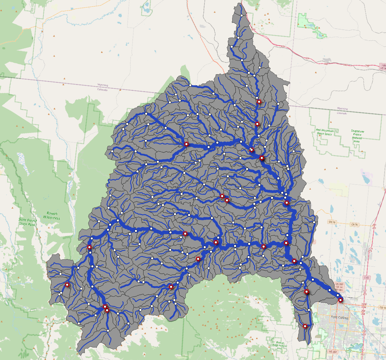

Let’s map it!

Defining the network

The exhaustive realization set (e.g identification and concepts) of a given network are contained in the network layer. This layer has no spatial information and is the link between all flowpath, divide, and nexus realizations contained within an area.

(net = read_sf(f, "network"))

## # A tibble: 1,884 × 15
##    id     toid  divide_id ds_id mainstem hl_id hydroseq hl_uri hf_source   hf_id
##    <chr>  <chr> <chr>     <dbl>    <int> <chr>    <int> <chr>  <chr>       <dbl>
##  1 wb-27… nex-… cat-2786…    NA   352913 788         NA HUC12… NA             NA
##  2 wb-27… nex-… cat-2786…    NA   352913 788      11238 HUC12… NHDPlusV2 2902759
##  3 wb-27… nex-… cat-2786…    NA   352913 788      11238 HUC12… NHDPlusV2 2900301
##  4 wb-27… nex-… cat-2786…    NA   352913 NA          NA NA     NA             NA
##  5 wb-27… nex-… cat-2786…    NA   352913 NA       11247 NA     NHDPlusV2 2900207
##  6 wb-27… nex-… cat-2786…    NA   352913 NA       11247 NA     NHDPlusV2 2900099
##  7 wb-27… nex-… cat-2786…    NA   352913 NA       11247 NA     NHDPlusV2 2900757
##  8 wb-27… nex-… cat-2786…    NA   352913 NA       11247 NA     NHDPlusV2 2900047
##  9 wb-27… nex-… cat-2786…    NA   352913 NA       11247 NA     NHDPlusV2 2900079
## 10 wb-27… nex-… cat-2786…    NA   352913 NA          NA NA     NA             NA
## # ℹ 1,874 more rows
## # ℹ 5 more variables: lengthkm <dbl>, areasqkm <dbl>,
## #   tot_drainage_areasqkm <dbl>, type <chr>, vpu <chr>

Notably, this file carries the full reference fabric, through manipulation, through data modeling steps. Here we see the “hf_source” (or reference fabric) was the NHDPlusV2.

The resulting 1884 row table stores the needed information for 420 divides, 590 flowpaths and 342 nexus

If a walk back to the source hf is not needed, a reduced set can be extracted, for example:

select(net, id, toid, divide_id, hl_uri, vpu, areasqkm) %>% 
  distinct()

## # A tibble: 606 × 6
##    id        toid       divide_id  hl_uri             vpu   areasqkm
##    <chr>     <chr>      <chr>      <chr>              <chr>    <dbl>
##  1 wb-278673 nex-278674 cat-278673 HUC12-101900070201 10L      13.3 
##  2 wb-278675 nex-278676 cat-278675 NA                 10L       7.44
##  3 wb-278676 nex-278677 cat-278676 NA                 10L       8.76
##  4 wb-278679 nex-278680 cat-278679 NA                 10L       4.52
##  5 wb-278680 nex-278681 cat-278680 NA                 10L       8.98
##  6 wb-278681 nex-278682 cat-278681 NA                 10L       6.63
##  7 wb-278682 nex-278683 cat-278682 NA                 10L      11.1 
##  8 wb-278683 nex-278684 cat-278683 NA                 10L       9.96
##  9 wb-278684 nex-278685 cat-278684 NA                 10L       8.61
## 10 wb-278686 nex-278687 cat-278686 NA                 10L      14.7 
## # ℹ 596 more rows

Forcing (Task 1)

To generate the forcing mesh (currently using EMSF) the forcing workstream needs the divide complex geometries and associated divide_id of each unit. These can be pulled directly from the divides layer!

read_sf(f, "divides") %>% 
  select(divide_id) %>% 
  filter(divide_id %in% net$divide_id)

## Simple feature collection with 419 features and 1 field
## Geometry type: MULTIPOLYGON
## Dimension:     XY
## Bounding box:  xmin: -831675 ymin: 1975605 xmax: -759465 ymax: 2061555
## Projected CRS: NAD83 / Conus Albers
## # A tibble: 419 × 2
##    divide_id                                                                geom
##  * <chr>                                                      <MULTIPOLYGON [m]>
##  1 cat-280570 (((-774075 2005635, -774375 2005635, -774345 2005695, -774345 200…
##  2 cat-278676 (((-822075 1993095, -822105 1992825, -822195 1992765, -822375 199…
##  3 cat-278680 (((-818235 2004705, -818265 2004585, -818355 2004585, -818625 200…
##  4 cat-278682 (((-810375 2006985, -810285 2006865, -810015 2006865, -809925 200…
##  5 cat-278683 (((-807825 2008065, -807705 2008005, -807555 2007825, -807495 200…
##  6 cat-278686 (((-794235 2002185, -794295 2002125, -794535 2002125, -794655 200…
##  7 cat-278689 (((-787395 2000865, -787575 2000715, -787575 2000595, -787665 200…
##  8 cat-278692 (((-778785 2002215, -778755 2002395, -778695 2002485, -778695 200…
##  9 cat-278693 (((-773565 1998705, -773625 1998615, -773745 1998585, -773865 199…
## 10 cat-278695 (((-767055 1994895, -767055 1994775, -766965 1994685, -766935 199…
## # ℹ 409 more rows

Rainfall Runoff Modeling (Task 2)

The NextGen rainfall runoff modeling tasks require the ability to identify a unit of the divide complex, and its associated draining flowpath. From this, configuration files can be used to assign and/or build model formulations associated with a given divide_id.

While NextGen remains a primarily lumped basin model, operating at the divide scale, the divide view is the ideal viewed realization. However, since we are not explicitly interested in geometries here, we drop them.

read_sf(f, "divides") %>%
  select(divide_id, id) %>%
  st_drop_geometry()

## # A tibble: 419 × 2
##    divide_id  id       
##  * <chr>      <chr>    
##  1 cat-280570 wb-280570
##  2 cat-278676 wb-278676
##  3 cat-278680 wb-278680
##  4 cat-278682 wb-278682
##  5 cat-278683 wb-278683
##  6 cat-278686 wb-278686
##  7 cat-278689 wb-278689
##  8 cat-278692 wb-278692
##  9 cat-278693 wb-278693
## 10 cat-278695 wb-278695
## # ℹ 409 more rows

NOTE: Had we used SQLite directly to access this layer, rather than reading the complete layer with sf, we could have avoided reading the geometry column entirely.

read_sf(f, query = "SELECT divide_id, id FROM divides")

## # A tibble: 419 × 2
##    divide_id  id       
##    <chr>      <chr>    
##  1 cat-280570 wb-280570
##  2 cat-278676 wb-278676
##  3 cat-278680 wb-278680
##  4 cat-278682 wb-278682
##  5 cat-278683 wb-278683
##  6 cat-278686 wb-278686
##  7 cat-278689 wb-278689
##  8 cat-278692 wb-278692
##  9 cat-278693 wb-278693
## 10 cat-278695 wb-278695
## # ℹ 409 more rows

Working across model formulations

Once divides are located, and models assigned, there is often a need to populate the configuration file with some pre-computed information. One example of this is operating the NOAH OWP Modular and CFE models which require a suite of divide-summarized data. This data lives adjacent to the core hydrofabric GPKG’s but can be accessed using a set of divide_id(s).

For example, let’s say we want CFE and NOAH OWP data for cat-280570, we can use the naming convention of our files, the network based VPU distinction, and general parquet/s3 access patterns.

base = 's3://nextgen-hydrofabric/pre-release'

open_dataset(glue("{base}/nextgen_{unique(net$vpu)}_cfe_noahowp.parquet")) %>%
  filter(divide_id == "cat-280570") %>%
  collect()

## # A tibble: 1 × 36
##   divide_id  gw_Coeff gw_Zmax gw_Expon `bexp_soil_layers_stag=1`
##   <chr>         <dbl>   <dbl>    <dbl>                     <dbl>
## 1 cat-280570    0.005    10.9        7                      9.01
## # ℹ 31 more variables: `bexp_soil_layers_stag=2` <dbl>,
## #   `bexp_soil_layers_stag=3` <dbl>, `bexp_soil_layers_stag=4` <dbl>,
## #   ISLTYP <int>, IVGTYP <int>, `dksat_soil_layers_stag=1` <dbl>,
## #   `dksat_soil_layers_stag=2` <dbl>, `dksat_soil_layers_stag=3` <dbl>,
## #   `dksat_soil_layers_stag=4` <dbl>, `psisat_soil_layers_stag=1` <dbl>,
## #   `psisat_soil_layers_stag=2` <dbl>, `psisat_soil_layers_stag=3` <dbl>,
## #   `psisat_soil_layers_stag=4` <dbl>, cwpvt <dbl>, mfsno <dbl>, mp <dbl>, …

Routing (Task 3)

Routing is based on the flowpath to nexus connection described in the background section and requires water to move from flowpaths, into nexuses, into flowpaths. More then one flowpath can contribute to a nexus, however only one nexus can contribute to a flowpath.

A hard requirement of ngen is that the network remains dendritic (e.g a DAG). We can ensure the resultant flowpath topology, extracted from the divides view, is compliant:

library(igraph); library(visNetwork)

## 
## Attaching package: 'igraph'

## The following objects are masked from 'package:dplyr':
## 
##     as_data_frame, groups, union

## The following objects are masked from 'package:stats':
## 
##     decompose, spectrum

## The following object is masked from 'package:base':
## 
##     union

g = select(net, id, toid) %>%
    distinct() %>% 
    graph_from_data_frame(directed = TRUE) 

is.dag(g)

## [1] TRUE

visIgraph(g)

Much like the NOAH-OWP/CFE example, knowing the connectivity of the flowpath network is half of the challenge. To successful route water through it, a range of attributes need to be supplied. Currently, these are provided within the flowpath_attributes layer of the hydrofabric data model:

read_sf(f, "flowpath_attributes") %>%
  filter(id %in% unique(net$id))

## # A tibble: 419 × 16
##    id       rl_gages rl_NHDWaterbodyComID    Qi  MusK  MusX      n      So ChSlp
##    <chr>    <chr>    <chr>                <dbl> <dbl> <dbl>  <dbl>   <dbl> <dbl>
##  1 wb-2786… NA       NA                       0  3600   0.2 0.06   0.0197  0.517
##  2 wb-2786… NA       NA                       0  3600   0.2 0.06   0.0214  0.438
##  3 wb-2786… NA       NA                       0  3600   0.2 0.055  0.0167  0.402
##  4 wb-2786… NA       NA                       0  3600   0.2 0.055  0.0193  0.365
##  5 wb-2786… NA       NA                       0  3600   0.2 0.0563 0.0489  0.452
##  6 wb-2786… NA       NA                       0  3600   0.2 0.055  0.0407  0.348
##  7 wb-2786… NA       NA                       0  3600   0.2 0.055  0.0340  0.329
##  8 wb-2786… NA       NA                       0  3600   0.2 0.055  0.0286  0.328
##  9 wb-2786… NA       NA                       0  3600   0.2 0.0556 0.0148  0.459
## 10 wb-2786… NA       NA                       0  3600   0.2 0.055  0.00464 0.316
## # ℹ 409 more rows
## # ℹ 7 more variables: BtmWdth <dbl>, time <dbl>, Kchan <dbl>, nCC <dbl>,
## #   TopWdthCC <dbl>, TopWdth <dbl>, length_m <dbl>

The id can be used to extract the complete/partial flowpath view if and when its needed:

fp = read_sf(f, "flowpaths") %>% 
  filter(id == net$id[1]) 

div = read_sf(f, "divides") %>% 
  filter(divide_id == net$divide_id[1])

mapview(div) + fp

Reporting (Task 4)

The last task is one that is NOT well facilitated by the existing NWM and that is how do you find the locations of known Points of Interest (POIs).

For example, lets say we wanted to find the USGS gages present in the Poudre Basin. To do this we could search the hydrolocations view for instances of type Gages.

(gages = filter(net, grepl("Gages", hl_uri)))

## # A tibble: 64 × 15
##    id     toid  divide_id ds_id mainstem hl_id hydroseq hl_uri hf_source   hf_id
##    <chr>  <chr> <chr>     <dbl>    <int> <chr>    <int> <chr>  <chr>       <dbl>
##  1 wb-27… nex-… cat-2786…    NA   352913 4447        NA Gages… NA             NA
##  2 wb-27… nex-… cat-2786…    NA   352913 4447     11598 Gages… NHDPlusV2 2899479
##  3 wb-27… nex-… cat-2786…    NA   352913 4447     11598 Gages… NHDPlusV2 2900683
##  4 wb-27… nex-… cat-2786…    NA   352913 4447     11598 Gages… NHDPlusV2 2899495
##  5 wb-27… nex-… cat-2786…    NA   352913 4447     11598 Gages… NHDPlusV2 2900705
##  6 wb-27… nex-… cat-2786…    NA   352913 4447     11598 Gages… NHDPlusV2 2900709
##  7 wb-28… nex-… cat-2805…    NA   376874 7845        NA Gages… NA             NA
##  8 wb-28… nex-… cat-2805…    NA   376874 7845     11527 Gages… NHDPlusV2 2898115
##  9 wb-28… nex-… cat-2805…    NA   376874 7845     11527 Gages… NHDPlusV2 2898115
## 10 wb-28… nex-… cat-2805…    NA   376874 7845     11527 Gages… NHDPlusV2 2898115
## # ℹ 54 more rows
## # ℹ 5 more variables: lengthkm <dbl>, areasqkm <dbl>,
## #   tot_drainage_areasqkm <dbl>, type <chr>, vpu <chr>

In total there are 15 gages in the Poudre River basin. If we want to map these, and their contributing flowpaths and divides, we simply need to walk across layers:

# Divides are indexed by divide_id
(div = read_sf(f, "divides") %>%
   filter(divide_id %in% gages$divide_id))

## Simple feature collection with 13 features and 9 fields
## Geometry type: MULTIPOLYGON
## Dimension:     XY
## Bounding box:  xmin: -828975 ymin: 1987995 xmax: -759465 ymax: 2027385
## Projected CRS: NAD83 / Conus Albers
## # A tibble: 13 × 10
##    divide_id  toid     type  ds_id areasqkm id    lengthkm tot_drainage_areasqkm
##  * <chr>      <chr>    <chr> <dbl>    <dbl> <chr>    <dbl>                 <dbl>
##  1 cat-278693 nex-278… netw…    NA     8.55 wb-2…     7.47               2734.  
##  2 cat-296532 nex-280… netw…    NA     8.40 wb-2…     5.21                 23.5 
##  3 cat-307431 nex-280… netw…    NA     4.40 wb-3…     3.89                  4.40
##  4 cat-307433 nex-280… netw…    NA    14.0  wb-3…     1.94                 14.0 
##  5 cat-280564 nex-280… netw…    NA     5.81 wb-2…     5.30                918.  
##  6 cat-280569 nex-280… netw…    NA     2.69 wb-2…     3.20               1395.  
##  7 cat-286396 nex-286… netw…    NA     6.35 wb-2…     5.34                240.  
##  8 cat-288037 nex-288… netw…    NA     6.88 wb-2…     2.64                 18.0 
##  9 cat-296529 nex-280… netw…    NA     4.38 wb-2…     3.45                 19.9 
## 10 cat-315473 nex-280… netw…    NA     4.36 wb-3…     2.23                  4.36
## 11 cat-331488 nex-286… netw…    NA     3.38 wb-3…     2.72                  3.38
## 12 cat-331480 nex-278… netw…    NA     3.10 wb-3…     3.40                  3.10
## 13 cat-278698 nex-278… netw…    NA     6.67 wb-2…     1.89               2966.  
## # ℹ 2 more variables: has_flowline <int>, geom <MULTIPOLYGON [m]>

# flowpaths are indexed by id
(fps = read_sf(f, "flowpaths") %>%
   filter(id %in% gages$id))

## Simple feature collection with 13 features and 10 fields
## Geometry type: MULTILINESTRING
## Dimension:     XY
## Bounding box:  xmin: -828149.9 ymin: 1989138 xmax: -759847.8 ymax: 2026467
## Projected CRS: NAD83 / Conus Albers
## # A tibble: 13 × 11
##    id      toid  mainstem order hydroseq lengthkm areasqkm tot_drainage_areasqkm
##  * <chr>   <chr>    <int> <dbl>    <int>    <dbl>    <dbl>                 <dbl>
##  1 wb-278… nex-…   352913     5    11598     7.47     8.55               2734.  
##  2 wb-280… nex-…   376874     4    11527     5.30     5.81                918.  
##  3 wb-280… nex-…   376874     4    11586     3.20     2.69               1395.  
##  4 wb-286… nex-…   461512     3    11338     5.34     6.35                240.  
##  5 wb-288… nex-…   486535     2    11215     2.64     6.88                 18.0 
##  6 wb-296… nex-…   622759     2    11404     5.21     8.40                 23.5 
##  7 wb-307… nex-…   785921     1    11405     3.89     4.40                  4.40
##  8 wb-296… nex-…   622754     2    11409     3.45     4.38                 19.9 
##  9 wb-315… nex-…   911271     1    11410     2.23     4.36                  4.36
## 10 wb-307… nex-…   785928     1    11585     1.94    14.0                  14.0 
## 11 wb-331… nex-…  1223251     1    11337     2.72     3.38                  3.38
## 12 wb-331… nex-…  1223233     1    11597     3.40     3.10                  3.10
## 13 wb-278… nex-…   352913     5    11627     1.89     6.67               2966.  
## # ℹ 3 more variables: has_divide <int>, divide_id <chr>,
## #   geom <MULTILINESTRING [m]>

# Nexus locations are indexed by toid
(hl = read_sf(f, "nexus") %>%
   filter(id %in% gages$toid))

## Simple feature collection with 6 features and 5 fields
## Geometry type: POINT
## Dimension:     XY
## Bounding box:  xmin: -826682 ymin: 1989138 xmax: -760037.4 ymax: 2023777
## Projected CRS: NAD83 / Conus Albers
## # A tibble: 6 × 6
##   id         toid      hl_id hl_uri              type                 geom
## * <chr>      <chr>     <chr> <chr>               <chr>         <POINT [m]>
## 1 nex-278694 wb-278694 4447  Gages-06752000      poi   (-771344.1 1998680)
## 2 nex-278699 wb-278699 8118  Gages-06752260      poi   (-760037.4 1989138)
## 3 nex-280565 wb-280565 7845  HUC12-101900070701… poi     (-779224 2023777)
## 4 nex-280570 wb-280570 8150  Gages-06751490      poi   (-773201.3 2012891)
## 5 nex-286397 wb-286397 7908  Gages-06748600      poi   (-794801.3 1999190)
## 6 nex-288038 wb-288038 8198  Gages-06746110      poi     (-826682 1992863)

mapview() + hl + div + fps

Conclusion

While there are many layers presented with a hydrofabric, all views can extracted through a combination of the network layer, and or through the “viewed” layer itself. This supplies everything needed to run ngen from start to finish, and allow introspection of the results!

It is able to do this through a clear implementation of HY Features concepts, within a detailed yet flexible data model. Taking advantage of this requires an understanding that:

the principle view of our data set is the flowpath network due to the topology requirements of both ngen and t-route. This means that flowpaths and nexus locations are uniquely identified by id, and divides are uniquely identified by divide_id.
viewing the divide “view” of the data still provides the ability to access the flowpath and nexus realizations by their identifiers,
auxiliary data can be built in relation to the appropriate realization (e.g. id, or divide_id) providing the ability for a larger data system to scaffold.

Mike Johnson

Justin Singh