The Reference Fabric
Mike Johnson
Lynker, NOAA-AffiliateDavid Blodgett
USGS WMAAndy Bock
USGS WMAAngus Watters
LynkerSource:
vignettes/02-design-deep-dive.Rmd
02-design-deep-dive.RmdHow do we arrive at the NextGen Hydrofabric?
The NextGen model engine is intended to be model agnostic.
The hydrofabric is meant to be Model Application Agnostic.
-
This means that the hydrofabric should be able to support the modeling needs of applications like:
- NOAA NextGen (in its infinite flavors);
- the USGS NHM;
- the USGS SPARROW model;
- and eventually NOAA FIM.
The USGS-NOAA Reference Fabric
For a single system to serve many - often distinct - modeling applications, there needs to be a set reference (analogous to a coordinate reference system (CRS))
-
This reference system must provide the maximum (e.g. smallest discretization) set of features “allowable” for all interrelated model applications.
- Right now, this is the NHDPlusV2 (with modifications)
- In the future it will move to NHDHighRes and 3DHP
- In practice, reference fabrics can be built from other hydrographies (e.g. NGA TDX and MERIT)
A reference fabric is key to providing persistent identification (PID) for durable data integration and model interoperability
The development of this product has been collaborative venture between the USGS Water Mission Area, the NOAA Office of Water Prediction, and Lynker.

More on this has been documented here
The 3 pillars of a Reference Fabric
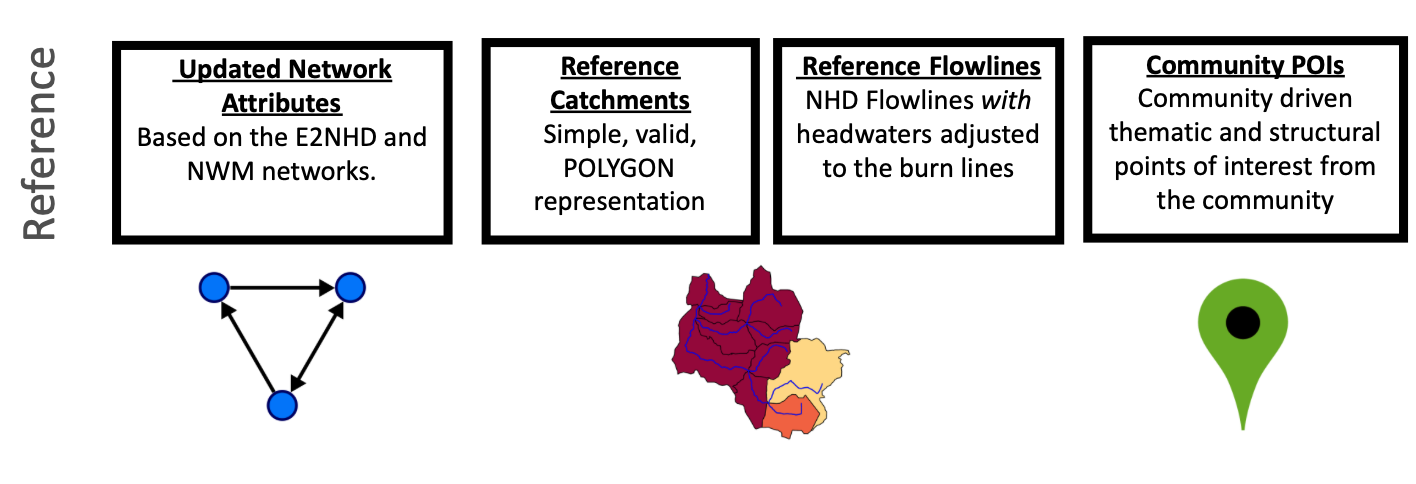
1. Reference Fabric
Simple, valid, representations of all
flowpathanddividefeaturesMust be derived from a source hydrographic dataset (e.g. NHDPlusV2, or Dihydro)
Currently, these are built out from the NHDPlusV2 features
Waterbodies are simplified, islands are dissolved, and they are unioned on GNIS_ID.

- Catchments are simplified, and DEM fragments are dissolved into the proper adjoining catchments.

Flowpaths are ensured to be digitized from upstream to downstream and the burn line events are substituted for the NHDFlowlines in headwater catchments
These data products can be foundhere
2. Reference Topology
Since its release, the NHDPlus topology and value added attributes have been stable
Local groups and agencies have made modifications to this but these have never made it back into the primary source
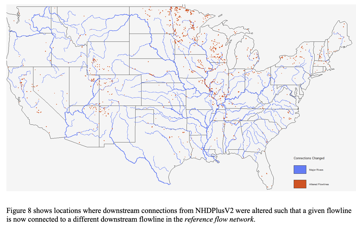
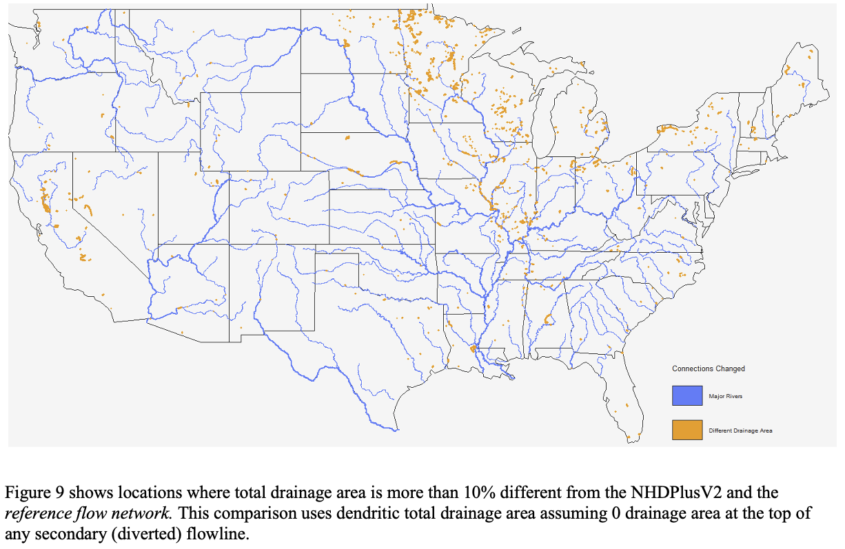
Improvements made by the USGS, OWP, NCAR and others have been integrated to provide an updated network connectivity.
This data product can be found here and is described in the upcoming article “Generating a reference flow network with improved connectivity to support durable data integration and reproducibility in the coterminous US” {In press at EMS}

3. Community Points of Interest (POI)
Points of Interest (POIs) for hydrologic modeling are collected from a variety of of published data sources. These include ones like the Army Corp National Inventory of Dams and the USGS Gages III gage database
POIs become
hydrolocationsat the outflow of the linkedflowpaththrough a robust hydrologic indexing scheme.NOTE: These are locations that have been deemed of high general interest. There is no guarantee all gages, dams, thermoelectric plants are in the community set.
What is a VPU?
A VPU is a Vector Processing Unit. The USGS determined these regions when designing the NHDPlusV2. Since our work builds off the NHDPlusV2, we adopt these processing units.
## Warning in st_point_on_surface.sfc(sf::st_zm(x)): st_point_on_surface may not
## give correct results for longitude/latitude data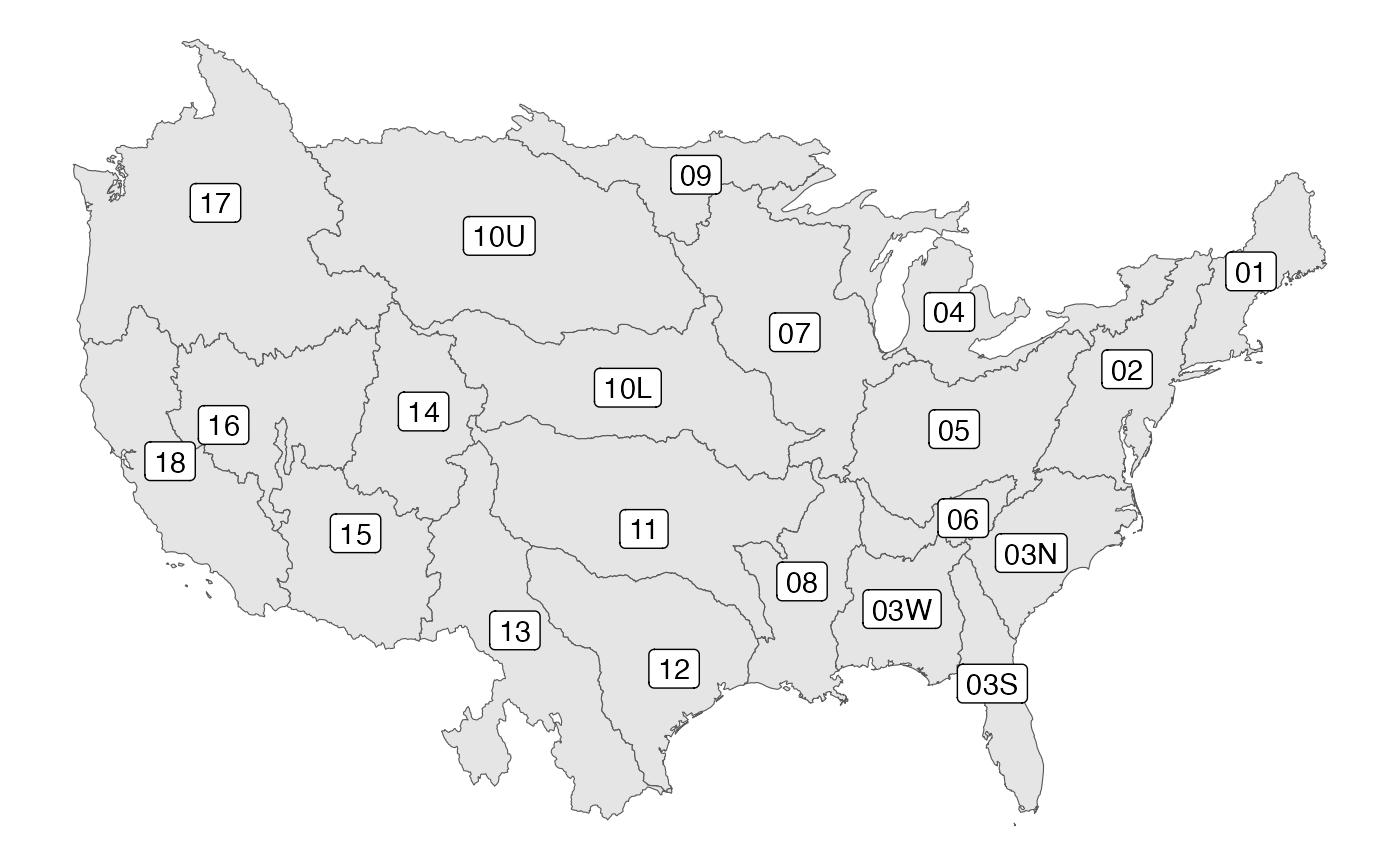
All hydrographic networks have VPU-esque discritizations. The key is that the source hydrofabric discritization can be retained through the manipulation process.
Below we show the tiling and drainage basin approaches of MERIT-hydro, BasinMaker, and NGA’s TDX-hydro.
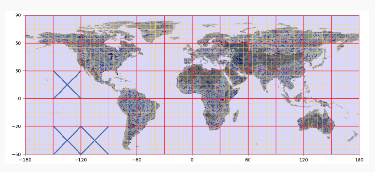
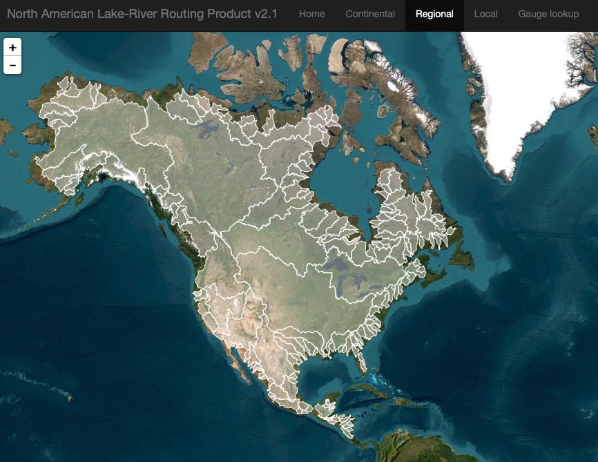
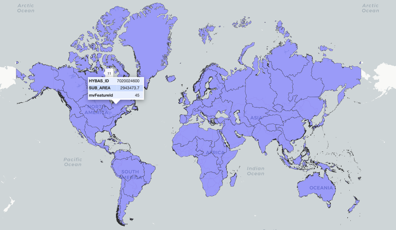
caption
Getting the reference fabric
All reference products live on Lynker Spatial s3 account.
They can be accessed with the web interface, downloaded, or interfaced with arrow.
The hydrofab::get_hydrofabric() utility will download
the most current geofabric for a Vector Processing Unit (VPU).
As an example, lets use the Geonconnex reference features to identify the location of our Fort Collins gage.
This location can be joined to the set of VPU boundaries severed with
nhdplusTools to find the correct VPU.
(gage = open_dataset('s3://lynker-spatial/hydrofabric/v2.2/conus_hl') |>
  select("vpuid", 'hl_reference', "hl_link") %>%
  filter(hl_link == '06752260') %>%
  collect())
## # A tibble: 2 × 3
## vpuid hl_reference hl_link
## <chr> <chr> <chr>
## 1 10L Gages 06752260
## 2 10L usgs_site_code 06752260
reference_gpkg = get_vpu_fabric(vpu = gage$vpuid[1],
                                outfile = glue("tutorial/vpu_{gage$vpuid[1]}.gpkg"))
## Warning in get_vpu_fabric(vpu = gage$vpuid[1], outfile =
## glue("tutorial/vpu_{gage$vpuid[1]}.gpkg")): tutorial/vpu_10L.gpkg already
## exists and overwrite is FALSEIf the requested file already exists, the file path will be returned.
Ok! With that, we have an idea of what the reference fabric is, how it was made, and how we can get it! The next stage is to learn how to manipulate this reference fabric for unique model applications.